26. Active filters

---

import numpy as np
import pandas as pd

import bokeh.plotting
import bokeh.io
bokeh.io.output_notebook()

Loading BokehJS ...

---

In a previous lesson, we built RC filters. Those filters were passive because they are not powered. Here, we will consider active filters, which feature powered op-amps.

Motivation for active filters

As we have already seen, the structure of a simple RC filter is the same as a voltage divider, as shown below.

For a low-pass filter, Z₁ is a resistor (say, with resistance \(R\)) and Z₂ is a capacitor (say, with capacitance \(C\)). In a high-pass filter, the Z₁ is a capacitor and Z₂ is a resistor.

Consider for a moment a low-pass RC filter. We previously worked out that

\begin{align} \left|V_\mathrm{out}\right| = \frac{1}{\sqrt{1 + \omega^2R^2C^2}}\,\left|V_\mathrm{in}\right|. \end{align}

To get a feel for this relationship, let’s make a plot of the response. The response is typically plotted in decibels (dB), given by

\begin{align} \text{dB} = 10 \log_{10}\frac{\left|V_\mathrm{out}\right|}{\left|V_\mathrm{in}\right|}. \end{align}

We plot the response in decibels below.

omega = np.logspace(-3, 3, 200)
lowpass_dB = -5 * np.log10(1 + omega**2)

p = bokeh.plotting.figure(
    frame_width=250,
    frame_height=175,
    x_axis_type='log',
    x_axis_label='ωRC',
    y_axis_label='response (dB)',
    x_range=[1e-3, 1e3],
    y_range=[-30, 1],
)

p.line([1e-3, 1, 1], [0, 0, -30], color='lightgray', line_width=4)
p.line(omega, lowpass_dB, line_width=2)

bokeh.io.show(p)

I have also included in this plot the response of an ideal low-pass filter in gray. Any frequencies above \(1/RC\) are blocked and those below \(1/RC\) can be passed through without significant attenuation. Conversely, the simple RC filter has a dull (as opposed to sharp) knee, the name given to the bend in the curve. To the right of the knee, the response features a roll off of ten dB per factor of ten in frequency.

We would like the response to be as close to ideal as possible. That means we want a steeper roll off. We also want the knee at \(\omega = 1/RC\) to be sharper. This can be accomplished with more complex filter designs, particularly through the use of inductors (giving so-called RLC filters).

There are, however, many disadvantages to using inductors. Importantly, they are bulky and expensive and also have series resistance, leading to non-ideal behavior. Fortunately, we can use op-amps to synthesize circuits that have the properties of (near) ideal RLC circuits. Because the op-amps are powered, these are called active filters.

Sallen-Key filters

We will consider one of the simplest active filters, the Sallen-Key filter. It is a simple special case of voltage-controlled voltage-source (VCVS) filters. The topology of the Sallen-Key filter is shown below.

For a high-pass filter, Z₁ and Z₂ are capacitors and Z₃ and Z₄ are resistors. For a low-pass filter, Z₁ and Z₂ are resistors and Z₃ and Z₄ are capacitors. The topology looks like cascaded RC filters, except with feedback.

Taking as an example a low-pass filter, we an take \(R_1 = R_2 = R\) and \(C_3 = C_4 = C\), and derive that the response is

\begin{align} \frac{\left|V_\mathrm{out}\right|}{\left|V_\mathrm{in}\right|} = \frac{1}{1 + \omega^2R^2C^2}. \end{align}

An important consequence of this result is that the cut-off frequency is, like in the case of the passive RC filters, about \(1/RC\). We can add this response to the plot.

sk_lowpass_dB = -10 * np.log10(1 + omega**2)
p.line(omega, sk_lowpass_dB, line_width=2, color='orange')

bokeh.io.show(p)

As you can see, the Sallen-Key filter has a steeper roll-off.

---

Thinking exercise 8: Sallen-Key response

Derive the above expression for the response of a Sallen-Key low-pass filter.

---

VCVS filters

Though the Sallen-Key filter has better roll-off, the knee, however, is still dull. This can be fixed by using the op-amp to amplify the output signal, as is done in VCVS filters, the topology of which is shown below.

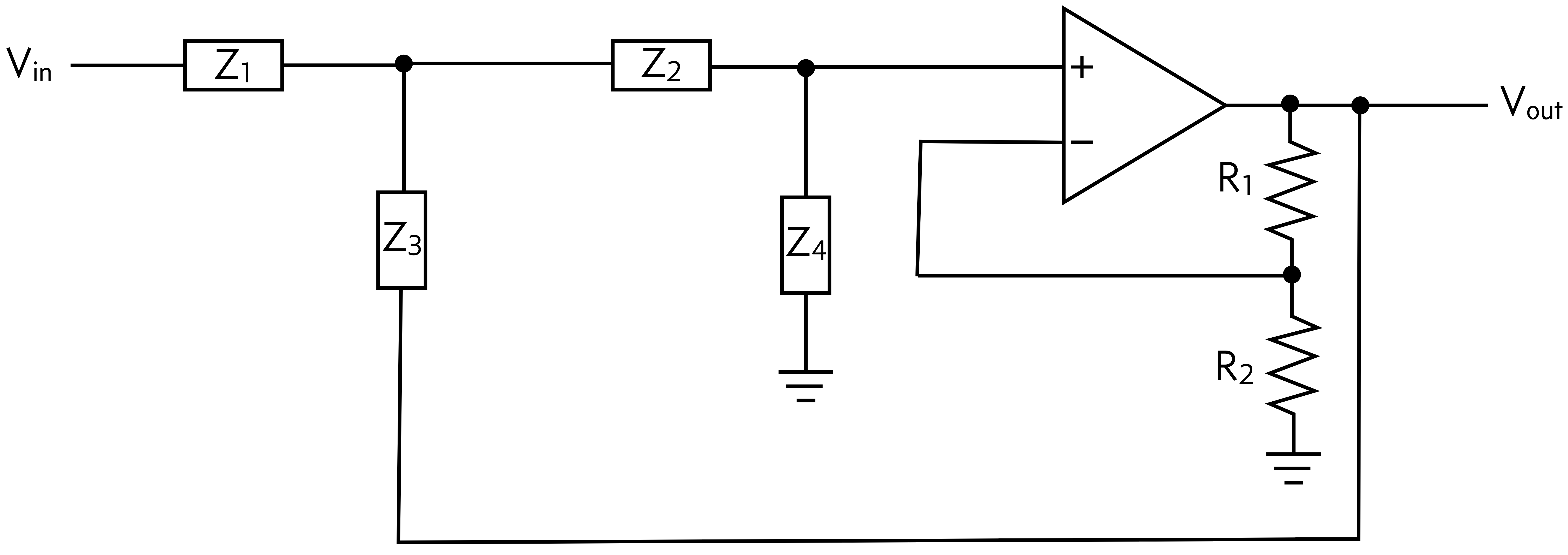
Within the VCVS topology many filters can be designed with sharp knees, strong roll-off, and flat pass bands. However, filter design requires careful thought, and things can go wrong, including introduction of ripple and resonance. I would recommend reading chapter 6 of Horowitz and Hill to learn more.

For the purposes of the projects in this class, you should be able to get good signals using a Sallen-Key filter, perhaps with some amplification after the filtering. (In looking at the above diagram, it is clear that the Sallen-Key filter is a VCVS filter with \(R_1 = 0\) and infinite \(R_2\).

Follow-along exercise 17: Sallen-Key filters

In this exercise, you will build two Sallen-Key filters, a high-pass one and a low-pass one. To see how they work, you will send a sinusoidal signal that is tainted with high-frequency noise that also has slow drift. The high-pass filter will eliminate the drift and the low-pass filter will eliminate the high-frequency noise.

Build the circuit below. The resistances are marked, and the capacitors should have capacitance \(C_1 = C_2 = 2.2\) µF and \(C_3 = C_4 = 0.22\) µF. Note that the part of the circuit featuring resistors R₁ and R₂ and capacitors C₁ and C₂ constitutes a high-pass filter, and the part of the circuit featuring R₃, R₄, C₃, and C₄ constitutes a low-pass filter.

Based on the resistor and capacitor values, we can plot the respective response curves for the respective filters. If you like, you can derive that the response curve for the high-pass filter is

\begin{align} \frac{\left|V_\mathrm{out}\right|}{\left|V_\mathrm{in}\right|} = \frac{1}{1 + \omega^{-2}R^{-2}C^{-2}}. \end{align}

# Resistances and capacitances
R = 68e3
C_lp = 0.22e-6
C_hp = 2.2e-6

omega = np.logspace(-3, 4, 200)
lowpass_dB = -10 * np.log10(1 + (2 * np.pi * R * C_lp * omega)**2)
highpass_dB = -10 * np.log10(1 + 1/(2 * np.pi * R * C_hp * omega)**2)

p = bokeh.plotting.figure(
    frame_width=300,
    frame_height=175,
    x_axis_type='log',
    x_axis_label='f (Hz)',
    y_axis_label='response (dB)',
    x_range=[1e-3, 1e4],
    y_range=[-30, 1],
)

p.line(omega, lowpass_dB, line_width=2, legend_label="low-pass")
p.line(omega, highpass_dB, line_width=2, color="orange", legend_label="high-pass")

p.legend.location = "bottom_center"

bokeh.io.show(p)

The high-pass filter lets frequencies above about 1 Hz through and the low-pass filter lets frequencies below about 10 Hz through. So, the low-pass filter should filter out high-frequency noise, and the high-pass filter should filter out slow variations in the signal.

To verify this, upload the sketch below to Arduino. The sketch is set up for use with serial-dashboard (time stamps are written out).

#include <Adafruit_MCP4725.h>

#define MCP4725_ADDR 0x62

const int analogOutPin = A0;
const int highPassPin = A1;
const int lowPassPin = A3;

const float highFreq = 10.0;
const float lowFreq = 0.1;
const unsigned long sampleDelay = 10;
const unsigned long dacDelay = 1;
unsigned long lastSampleTime = 0;
unsigned long lastDACTime = 0;

Adafruit_MCP4725 dac;

unsigned long printVoltages() {
  unsigned long timeMilliseconds = millis();

  // Read voltages
  int dacReading = analogRead(analogOutPin);
  int highPassReading = analogRead(highPassPin);
  int lowPassReading = analogRead(lowPassPin);

  // Write the result
  if (Serial.availableForWrite()) {
    Serial.print(timeMilliseconds);
    Serial.print(",");
    Serial.print(dacReading);
    Serial.print(",");
    Serial.print(highPassReading);
    Serial.print(",");
    Serial.println(lowPassReading);
  }

  // Return time of acquisition
  return timeMilliseconds;
}


void setup() {
  dac.begin(MCP4725_ADDR);

  Serial.begin(115200);
}


void loop() {
    unsigned long currTime = millis();

  if (currTime - lastDACTime > dacDelay) {
    // Middle frequency signal
    int xMid = (int)(1000 * (1 + sin(2 * PI * highFreq * millis() / 1000.0)) / 2.0);

    // Slowly varying drift
    int xLow = (int)(1000 * (1 + sin(2 * PI * lowFreq * millis() / 1000.0)) / 2.0);

    // High-frequency noise
    int xRand = (int)(random(0, 2000) - 500);

    // Set the output
    dac.setVoltage((uint16_t) max(min(xLow + xMid + xRand, 4095), 0), false);
  }

  if (currTime - lastSampleTime > sampleDelay) {
    lastSampleTime = printVoltages();
  }
}

The first column outputted is the time stamp in milliseconds. The second is the voltage that goes into the filters (a blue line in serial-dashboard). The second is the output of the high-pass filter (an orange line). The third is the output of the low-pass filter (a green line).

Look at the signals coming out. Are the filters working as expected?

---

Do-it-yourself exercise 13: A bandpass filter

A bandpass filter allows intermediate frequencies through while filtering out high and low frequencies. They can be constructed by using a high-pass filter followed by a low-pass filter. In the case of the filters we have just considered, you can take the output of the high-pass filter and make that the input of the low-pass filter. Your task in this exercise is to implement that and see if you get the expected signal. There will be some attenuation, you should amplify the output of the bandpass filter.

---

Note that we are just scratching the surface of filter design here. It is a rich and interesting field and you can create all kinds of filters with useful properties. What we have shown here for making low-, high-, and bandpass filters is only one (and a rather simple one) of myriad ways of filtering signals.